Hands-On Session

In the following, we will guide you through all the steps required to model, deploy, and execute a hybrid quantum application using workflows. In the first part of the tutorial, a quantum workflow is modeled manually by attendees. Afterwards, the same workflow is automatically generated based on a set of selected patterns.

The use case utilizes the following tools:

• Pattern Atlas: A graphical tool for authoring and visualizing patterns and pattern languages.
• Process View Plugin: A plugin for the Camunda engine to visualize process views.
• OpenTOSCA Container: A TOSCA-compliant deployment system.
• Quantum Workflow Modeler: A graphical BPMN modeler to define, transform, and deploy quantum workflows.
• Quokka: A microservice ecosystem enabling a service-based execution of quantum algorithms.
• Winery: A web-based modeler for TOSCA-based deployment models, which can be attached to activities of quantum workflows to enable their automated deployment in the target environment.

Setup

In case you participate in the tutorial on-site and use one of the provided virtual machines, move to Part 1 and use the provided IP to replace the placeholder $IP.

The code required for the hands-on session is available here.

On Windows, you have to activate long paths for Git to enable cloning and pushing to this repository. Thus, execute the following command:

git config --system core.longpaths true

Afterwards, clone the repository and navigate to the 2024-icwe-tutorial folder:

git clone https://github.com/UST-QuAntiL/QuantME-UseCases.git
cd QuantME-UseCases/2024-icwe-tutorial

All components are available via Docker. Therefore, these components can be started using the Docker-Compose file available here:

1. Update the .env file with your settings:
   • PUBLIC_HOSTNAME: Enter the hostname/IP address of your Docker engine. Do not use localhost.
   • IBM_ACCESS_TOKEN: Enter your IBMQ token, which can be retrieved here. The token can also be left empty, but then the views described below only display a reduced set of data.
2. Run the Docker-Compose file:

   cd docker
   docker-compose pull
   docker-compose up --build
   

3. Wait until all containers are up and running. This may take some minutes.

Quantum Workflow Modeler

Open the quantum workflow modeler using the following URL: http://$IP:1893

Afterwards, the following screen should be displayed:

Familiarize yourself with the workflow modeler by dragging and dropping elements from the palette on the right into the modeling pane.

If you are not familiar with BPMN, have a look at the Camunda introduction.

Part 1: QAOA for MaxCut

In the first part of the hands-on session, you will model and execute a quantum workflow orchestrating the Quantum Approximate Optimization Algorithm (QAOA) to solve the Maximum Cut (MaxCut) problem. To model the quantum workflow, the Quantum Modeling Extension (QuantME) is used.

Please download the initial workflow model available here. It contains a pre-configured Start Event requesting the required input for the workflow execution. Open the workflow model by clicking on File and Open File. Afterwards, proceed with the following steps to model and execute the quantum workflow orchestrating QAOA:

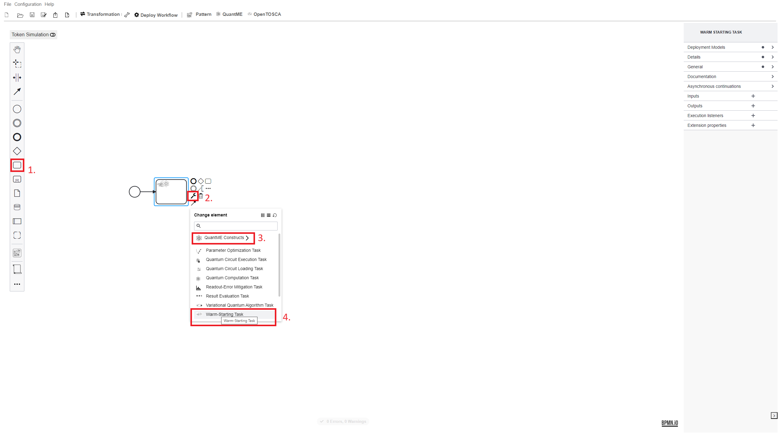
1. Add a Warm-Starting Task after the Start Event. Warm-starting is used to approximate a solution that is incorporated into the quantum circuit to facilitate the search for the optimal solution. Select the Task icon in the palette (1), drag it into the pane, click on the wrench symbol (2), then first select the QuantME Constructs category, and afterwards QuantME Tasks in the drop-down menu (3). Finally, click on Warm-Starting Task within the QuantME Tasks category (4).

   

2. Configure the Warm-Starting Task using the values shown below. Thereby, Biased Initial State is selected as Warm-Starting pattern and Initial State Warm-Start Egger as Warm-Starting method. Furthermore, we will use QAOA to solve the MaxCut problem, thus, select QAOA as the quantum algorithm to warm-start. Finally, utilize the Goemans-Williamson algorithm to calculate the initial state to use, as well as 10 repetitions to use for the approximation.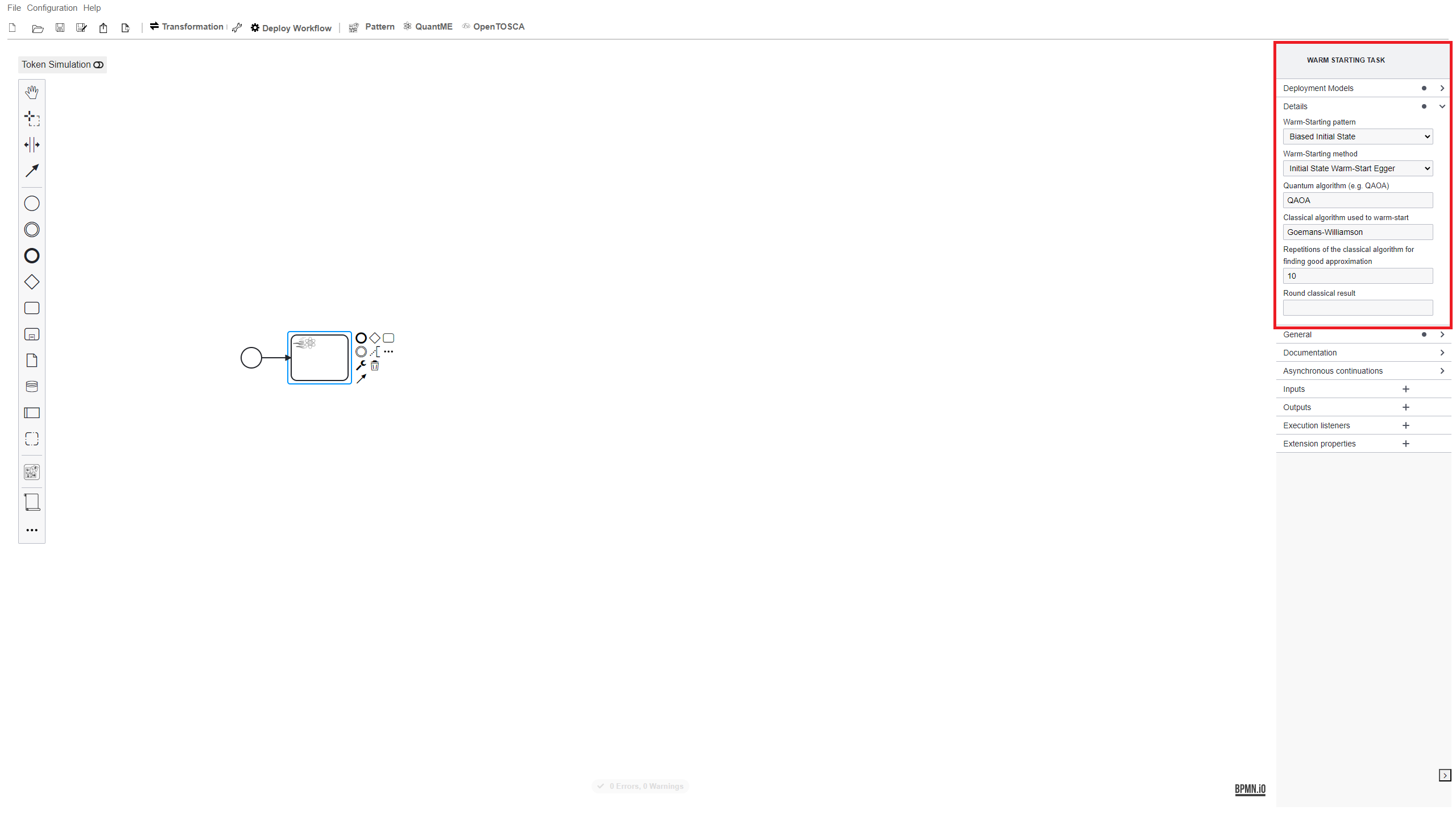

   

3. Next, add a second task of type Quantum Circuit Loading Task to load to parameterized QAOA circuit that is later executed in the variational loop. The functionality to generate a corresponding quantum circuit is provided by Quokka, therefore, configure the task using quokka/maxcut as URL. Furthermore, connect both tasks with the start event using sequence flow.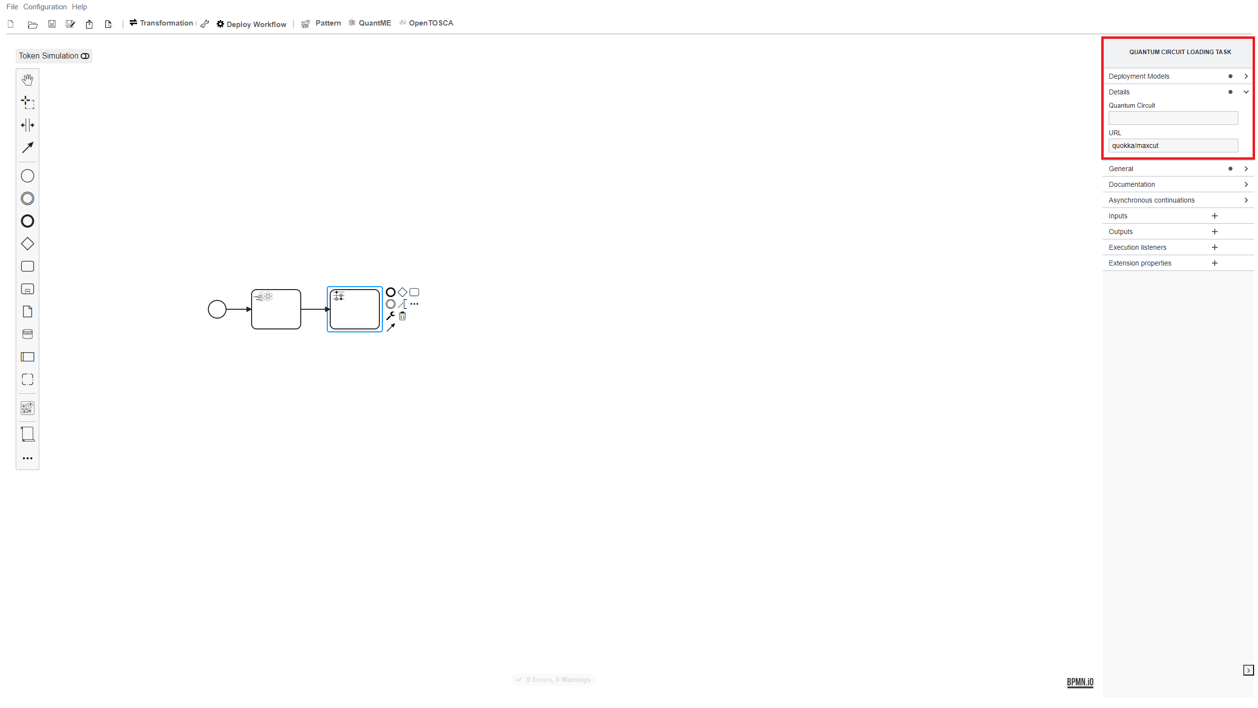

   

4. Due to today’s restricted quantum computers, the quantum circuit should be cut into multiple smaller sub-circuits, thus, reducing the impact of errors, as well as the limited number of qubits. Add a Circuit Cutting Task, which is also available within the QuantME Tasks category. Configure the Circuit Cutting Task to use the Cutting Method knitting toolbox, utilizing the implementation provided by the Circuit Knitting Toolbox. Furthermore, set the Maximum Sub-Circuit width to 4, the Maximum Number of Cuts to 2, and the Maximum Number of Sub-Circuits to 2. Finally, add an Exclusive Gateway to later join the sequence flow of the optimization loop.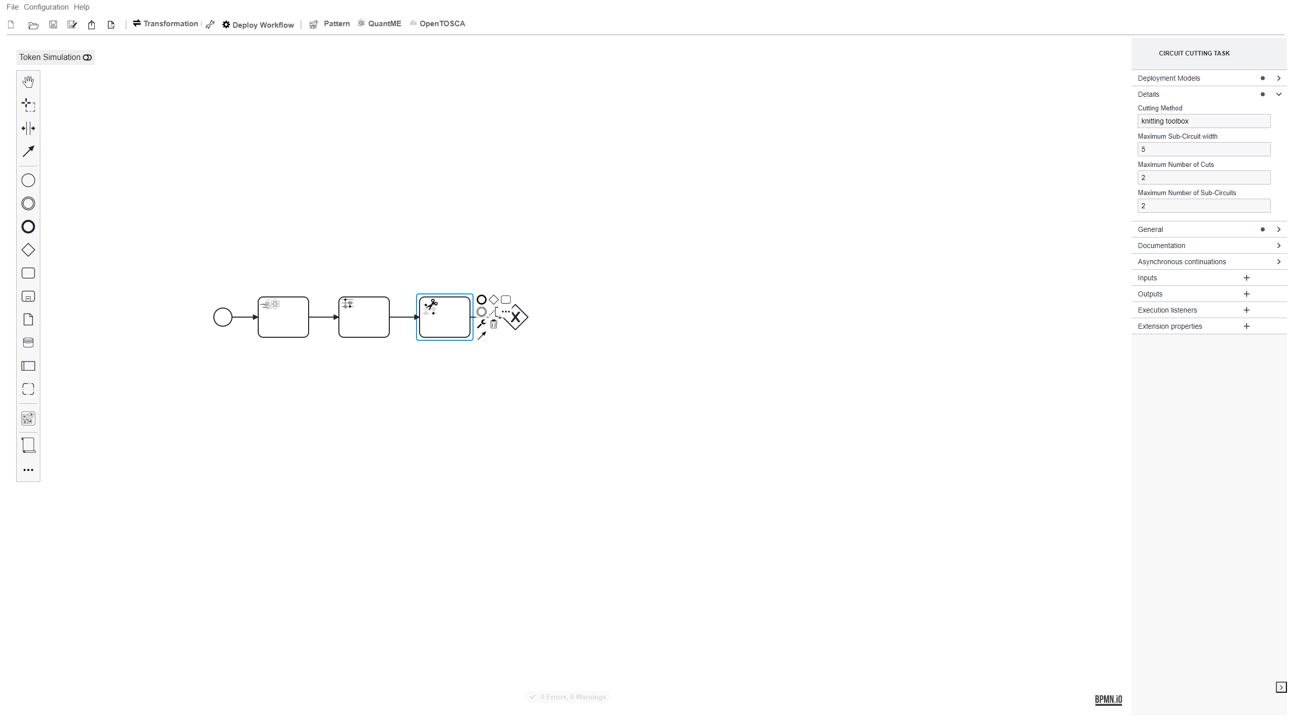

   

5. Next, add a task of type Quantum Circuit Execution Task to execute the loaded quantum circuit on a quantum computer. For this example, we configure the task to use ibm as the quantum hardware provider and the aer_qasm_simulator as QPU. The aer_qasm_simulator is a simulator that can be executed locally to avoid queuing times. Furthermore, the number of shots, i.e., the number of executions, is set to 2000, and it is specified that the circuit to execute was implemented using openqasm.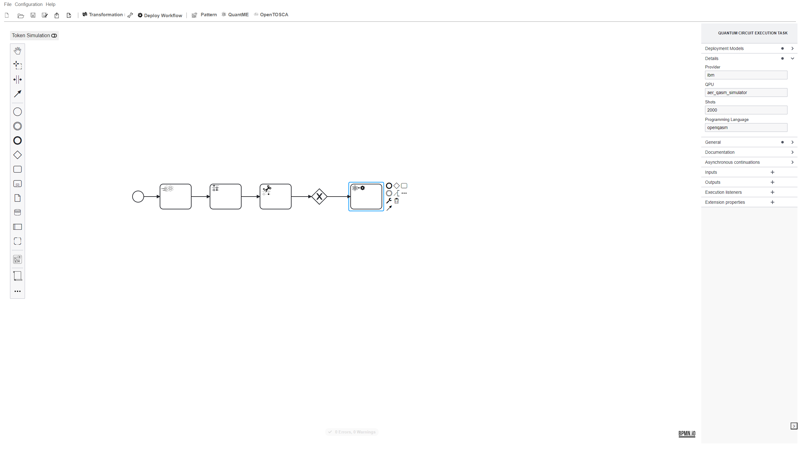

   

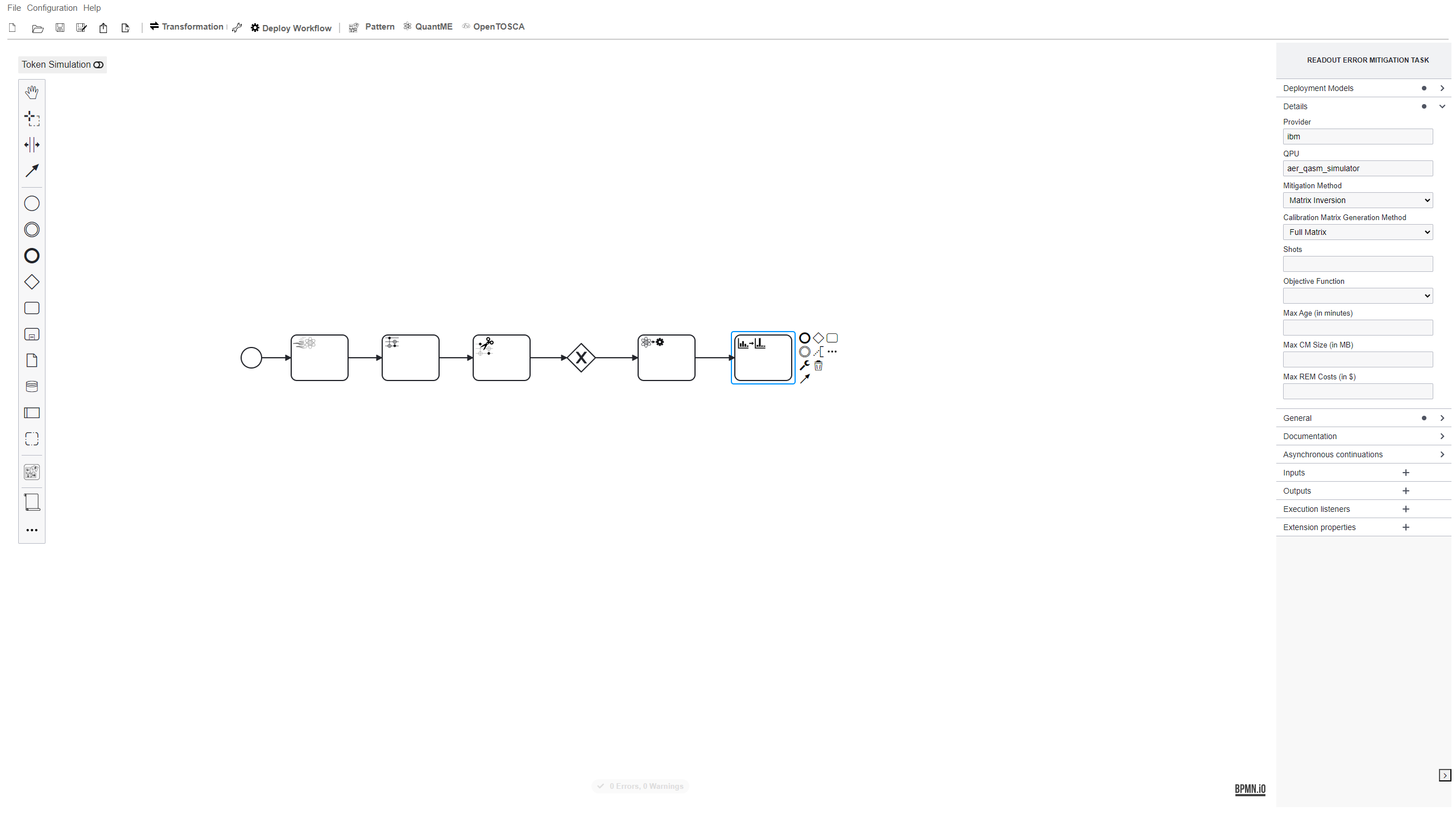
6. To reduce the impact of readout errors, add a Readout Error Mitigation Task and configure it as follows:
   • Provider: ibm
   • QPU: aer_qasm_simulator
   • Mitigation Method: Matrix Inversion
   • Calibration Matrix Generation Method: Full Matrix

   

7. After the mitigation, the results of the different sub-circuit executions are combined using a Cutting Result Combination Task to receive the overall result. Thereby, the same Cutting Method must be used, i.e., knitting toolbox.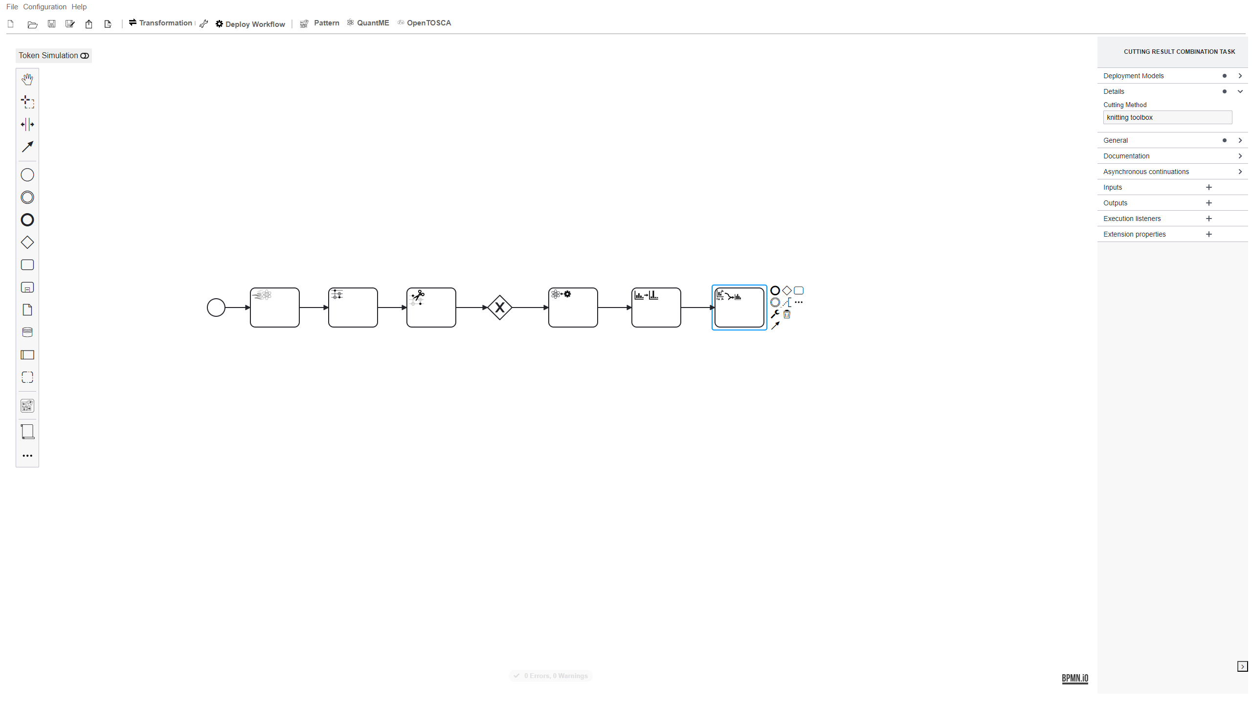

   

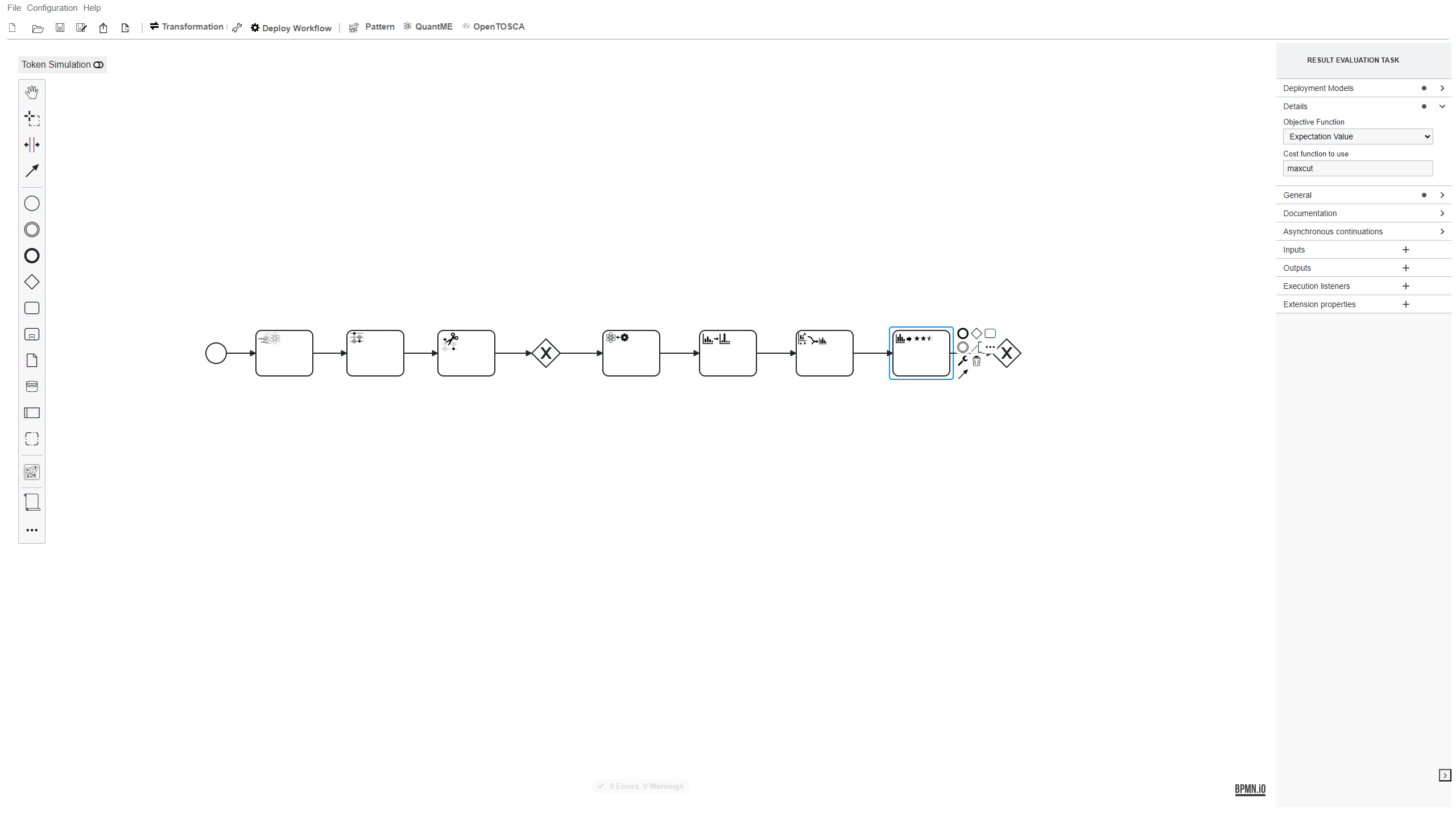
8. To evaluate the quality of the results, add a Result Evaluation Task and configure it as follows:

   • Objective Function: Expectation Value
   • Cost function to use: maxcut

   Additionally, add another Exclusive Gateway to enter the next iteration of the optimization loop if required.

   

9. If another iteration is required, the parameters are optimized using a Parameter Optimization Task. Configure the task to utilize Cobyla as an Optimizer.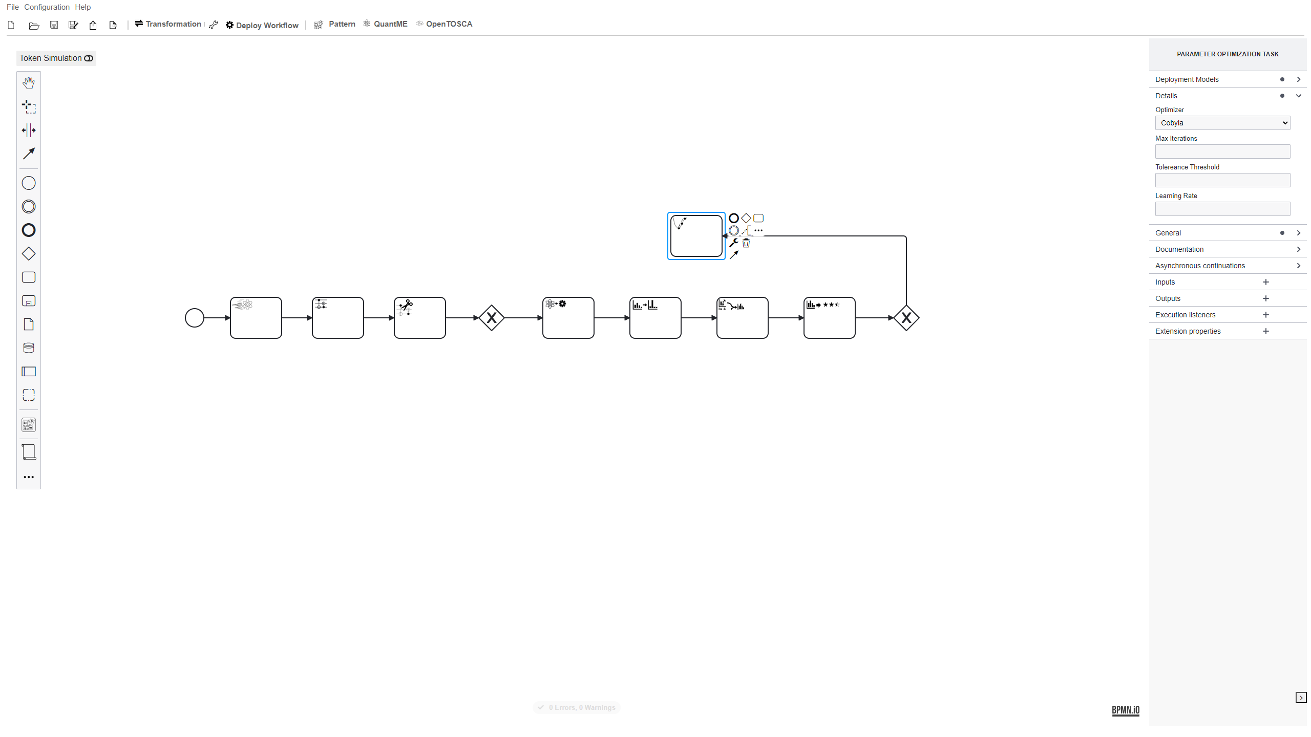

   

10. Connect the Optimizer Task to the first Exclusive Gateway. Afterwards, add the following expression to the sequence flow between the second Exclusive Gateway and the Optimizer Task as shown below: ${ execution.getVariable('converged')== null || execution.getVariable('converged') == 'false'}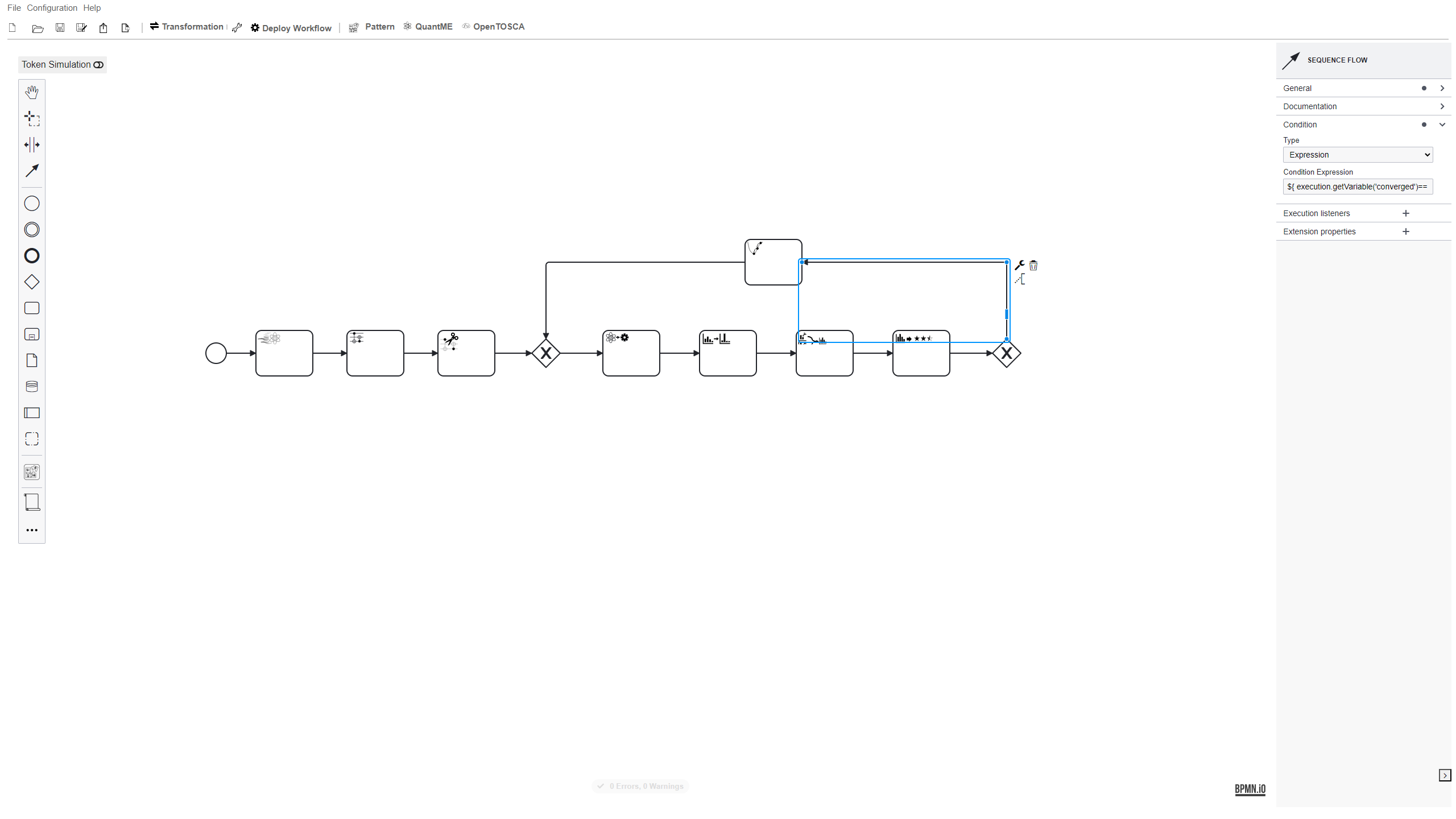

    

11. Finally, add a User Task and connect the second Exclusive Gateway to it. Furthermore, use the following condition: ${ execution.getVariable('converged')!= null && execution.getVariable('converged') == 'true'} The Result Evaluation Task generates an image to visualize the identified MaxCut. Thus, the User Task has to be configured to enable analyzing this image. Hence, use a form of type Generated Task Forms and add a form field to display the URL of the result image as shown below: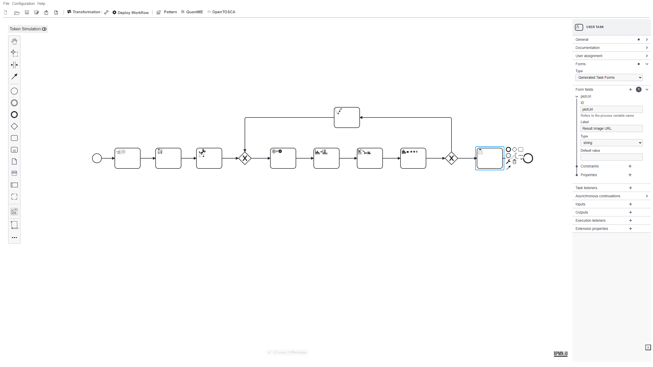

    

12. To execute the workflow, the QuantME modeling constructs must be replaced by standard-compliant BPMN modeling constructs. Therefore, click on the Transform button. The resulting native workflow model is displayed below. For example, the Warm-Starting Task and Quantum Circuit Loading Task are replaced by two Service Tasks invoking the corresponding services of the Quokka ecosystem based on the configuration attributes.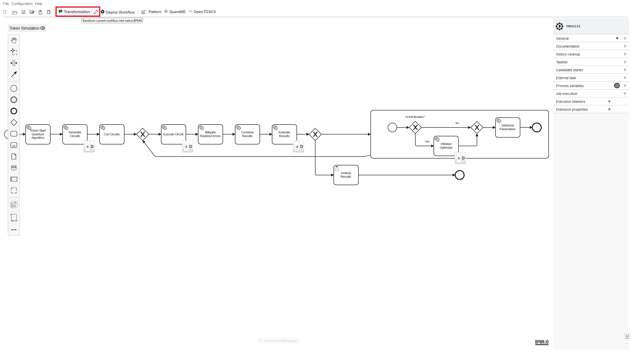

    

13. In case you experience any problems, the workflow model after transformation is available here, which can be opened in the modeler to continue from this point.

    Next, the required services to execute the workflow model must be deployed. For this, deployment models are attached to the activities of the workflow, enabling to deploy the services for these activities. Click on the OpenTOSCA button and then select Service Deployment. The popup shows the services that have to be deployed. Click on Upload CSAR to start the deployment process. In case you participate in the tutorial on-site and use one of the provided virtual machines, the services are already pre-deployed and are directly bound to the workflow. Otherwise, please follow the steps of the deployment dialogue.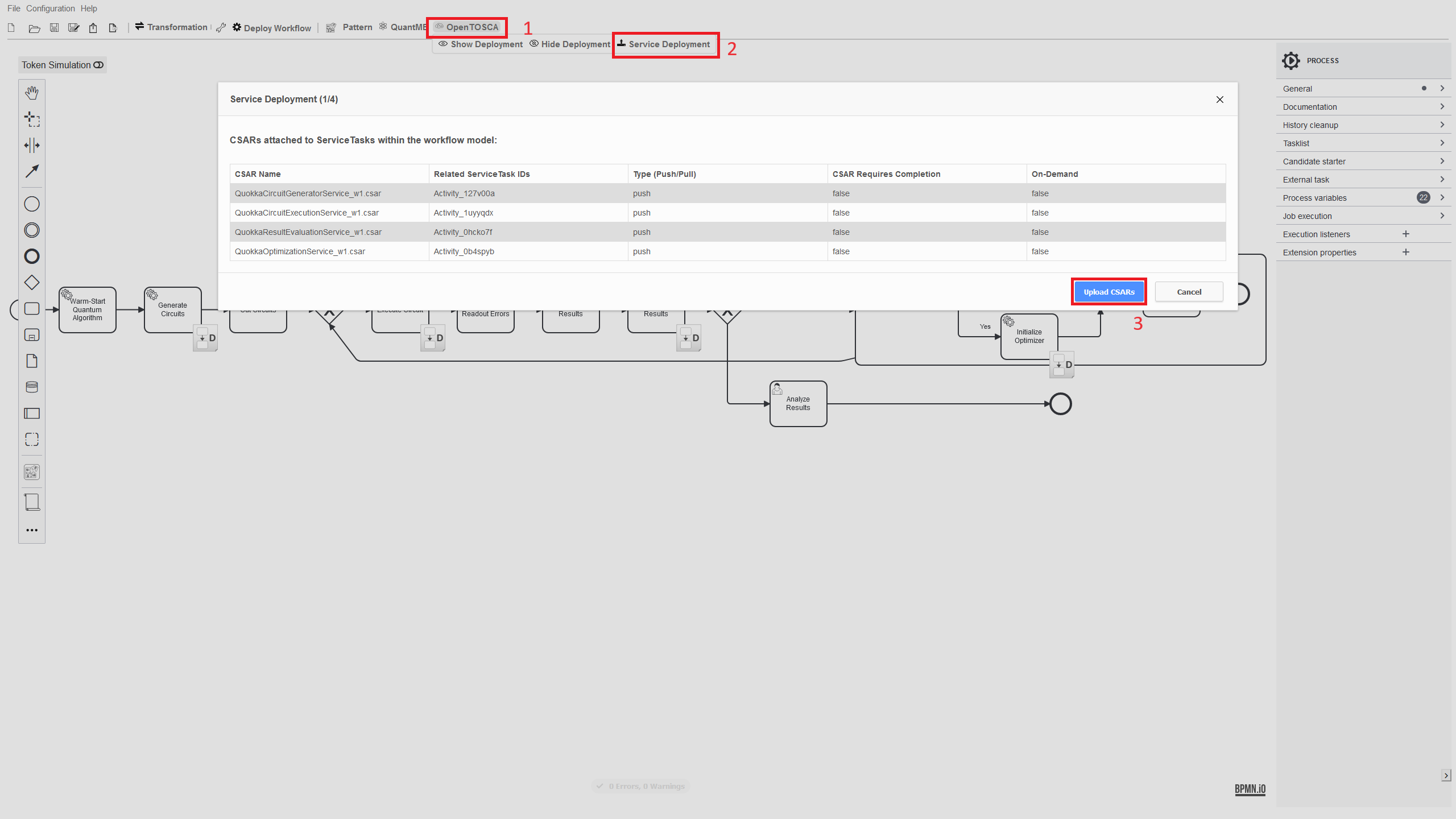

    

14. After the binding completes, a corresponding notification is displayed as shown below. Finally, to upload the workflow to the Camunda Engine, click on the Deploy Workflow button: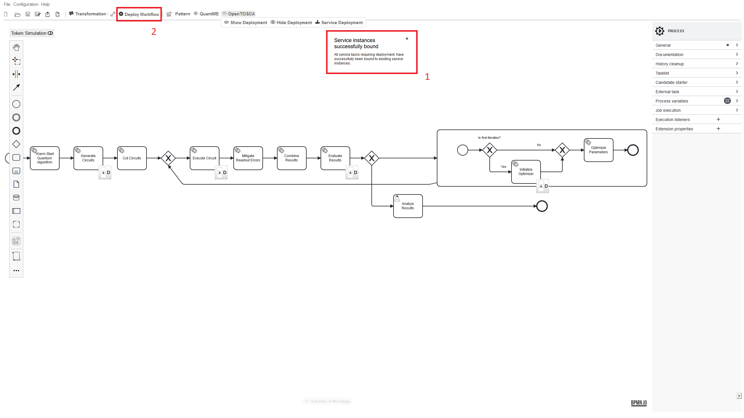

    

15. Open the Camunda Engine using the following URL: http://$IP:8090 Use demo as username and password to log in, which displays the following screen: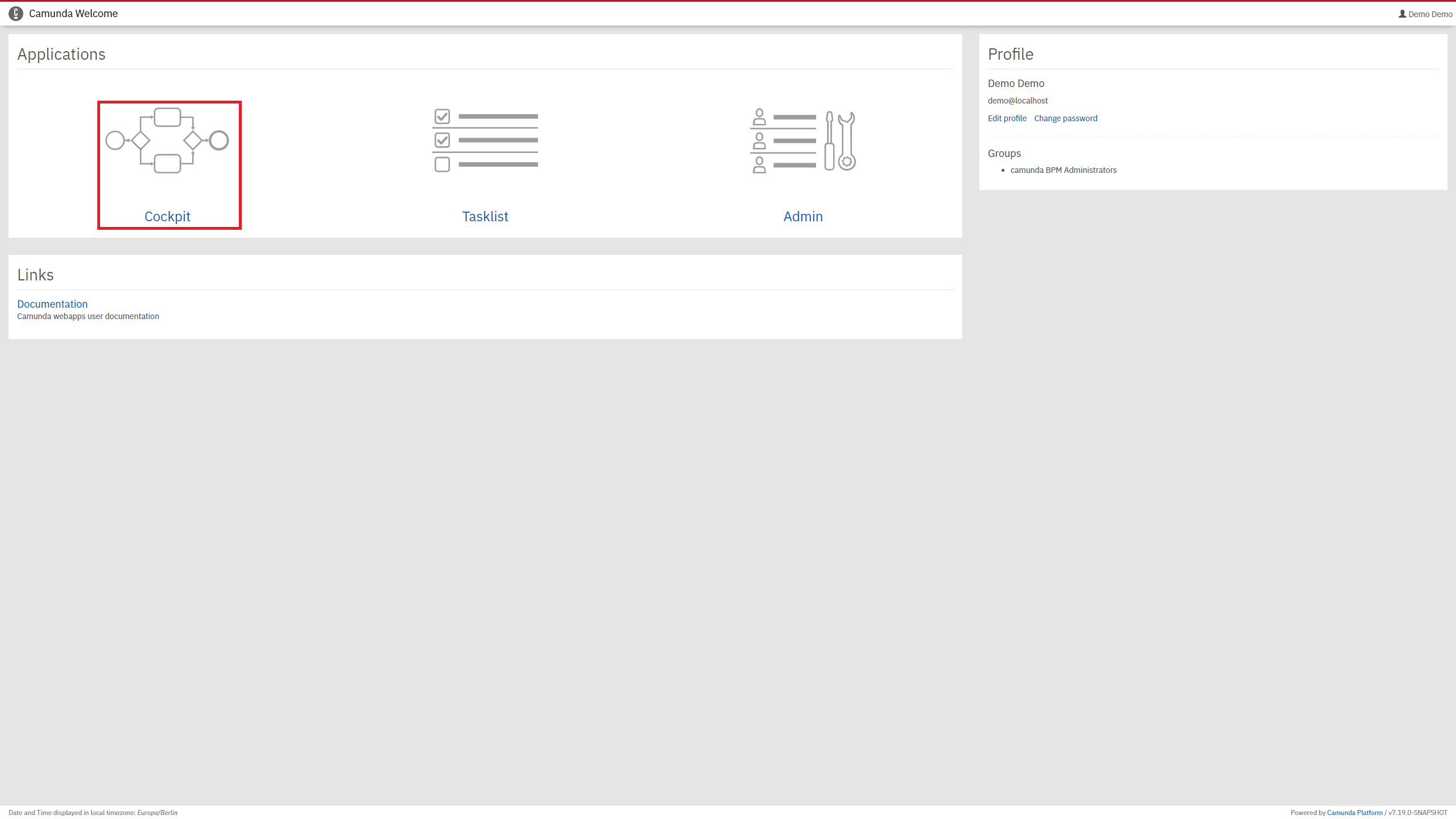

    

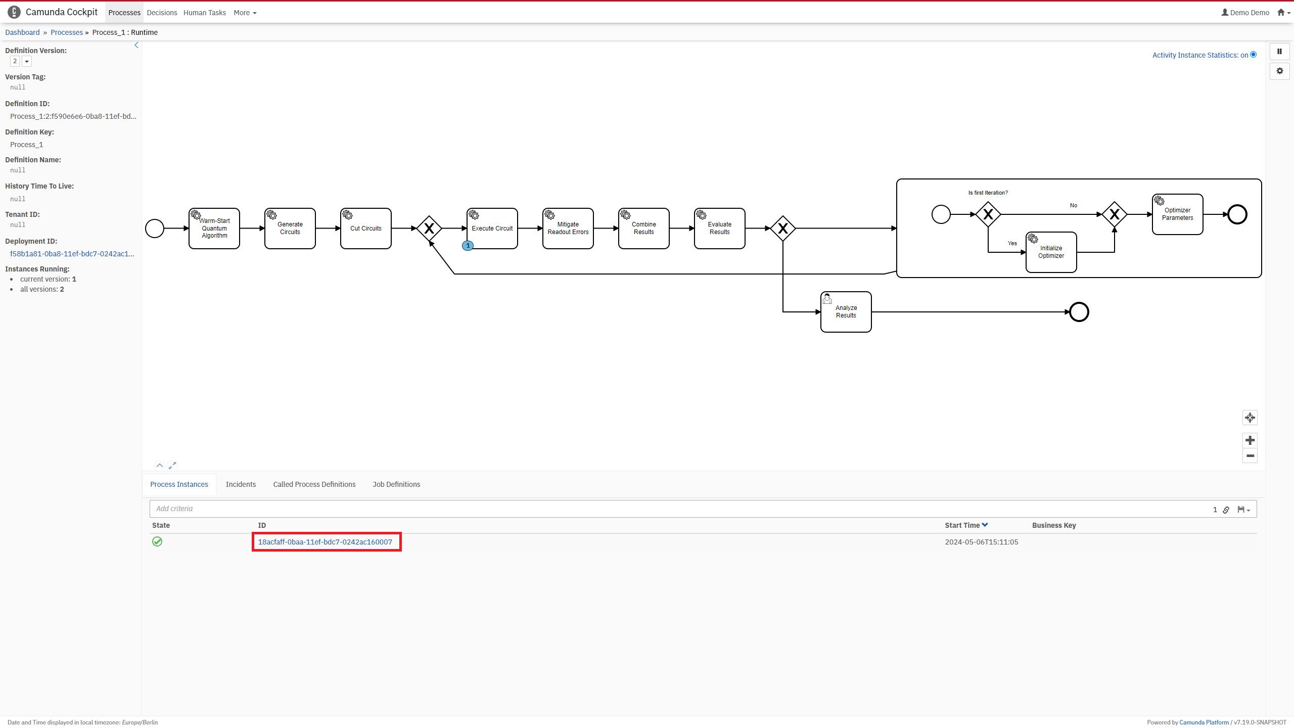
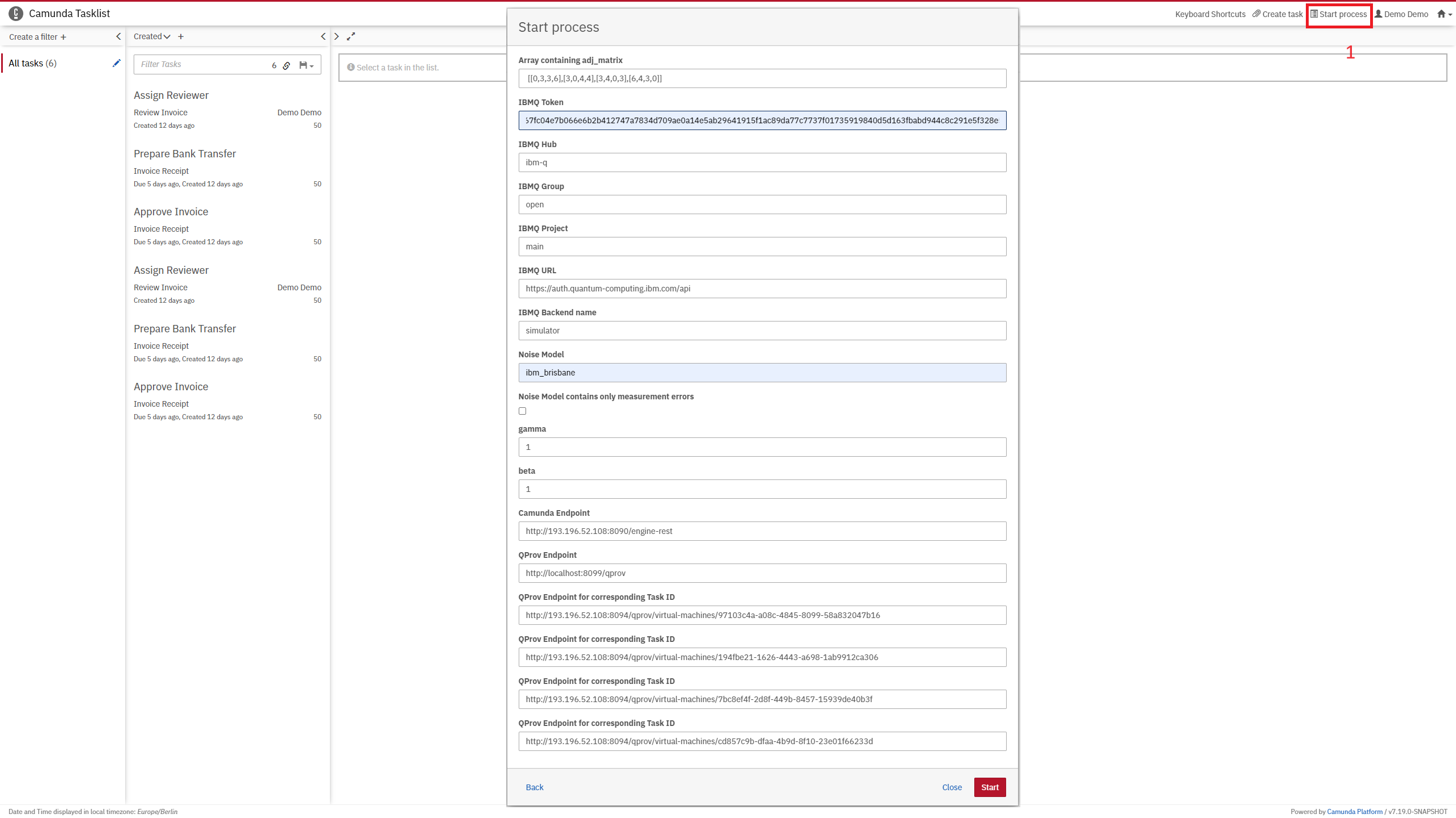
16. Click on Cockpit to validate that the workflow was successfully uploaded. Then, click on Processes on the top-left and select the workflow from the list.

    This should show a graphical representation of the uploaded workflow. To instantiate the workflow, click the home button on the top-right, then select Tasklist. Next, click on Start process on the top-right, select the name of the uploaded workflow, and provide the input parameters as shown below:

    • IBMQ Token: Enter your IBMQ token, which can be retrieved here.
    • Noise Model: Provide the name of a QPU to use the corresponding noise model for the simulator. In the example, we use ibm_brisbane.

    

17. Switch back to the Camunda Cockpit, and select the deployed workflow. Then, a running process instance should be shown on the bottom. Click on the ID of the instance to visualize the current variables, as well as the position of the token. Check the variables to trace the current iteration, as well as costs of the optimization process. Reload the Camunda Cockpit periodically to observe the current progress.

    

18. To activate the quantum view, visualizing the QuantME modeling constructs, as well as quantum-specific provenance data, such as calibration data of the QPU, click on toggle quantum view on the right. Hover over the different QuantME modeling constructs to visualize additional, task-specific data: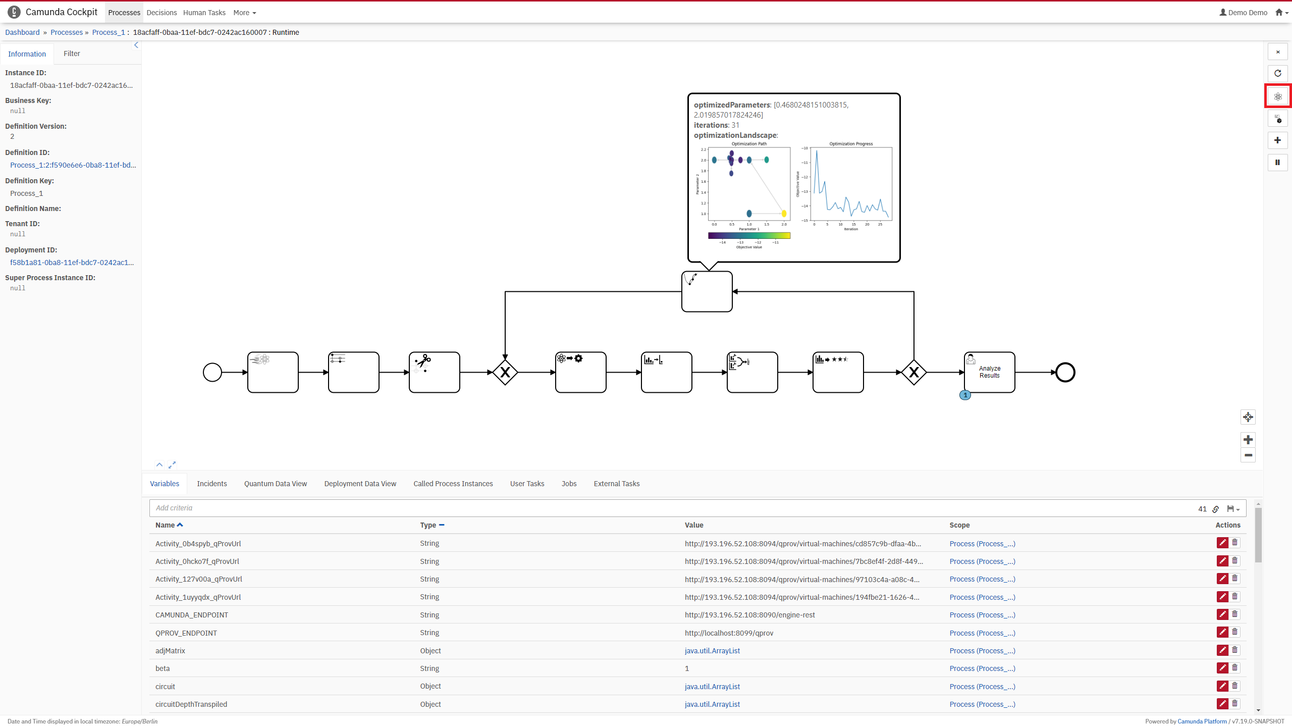

    

19. Wait until the token reaches the final user task (reload the Camunda Cockpit periodically), then, switch to the Tasklist. Select the task item on the left, then click on Claim to activate the item, and download the result plot using the given URL. Afterwards, click on Complete to terminate the workflow instance. Finally, open the downloaded image, visualizing the MaxCut solution for the input graph.

Part 2: Pattern-based Generation of Quantum Workflows

In the second part of the tutorial, we will discuss how to simplify the modeling process, by automatically generating the quantum workflow modeled in the first part based on a set of selected patterns. Therefore, we utilize the quantum computing patterns.

Please proceed with the following steps to generate, adapt, and execute the quantum workflow using patterns:

1. Click on Pattern and afterwards on Open Pattern Selection. For the generation of quantum workflows, we distinguish three categories of patterns: (i) Algorithm patterns, enabling to choose the quantum algorithms that should be orchestrated by the quantum workflow. (ii) Behavioral patterns, determining the execution strategy for the chosen algorithms, e.g., by using a hybrid runtime or a session. (iii) Augmentation patterns, supporting the enhancement of the quantum workflow by incorporating additional features or elements, such as warm-starting or circuit cutting. Click on the Select Patterns button to start the pattern selection for the use case.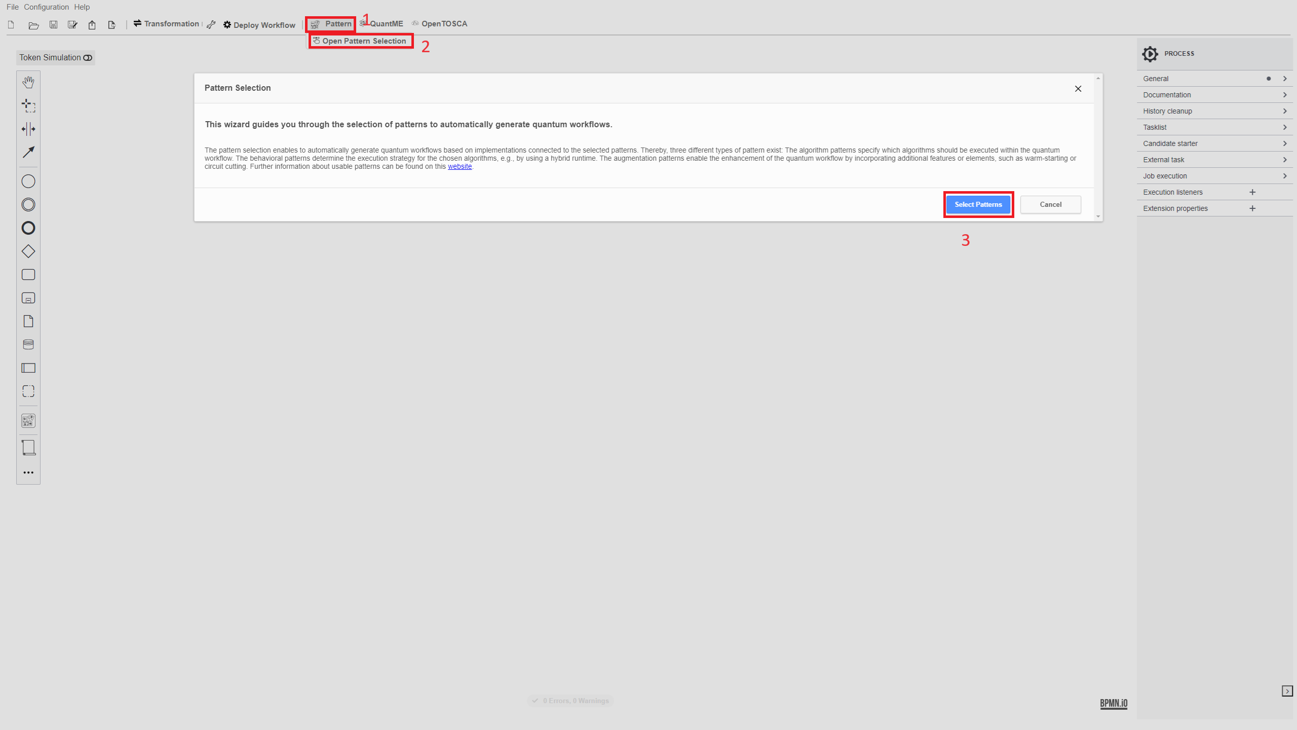

   

2. Click on the + sign on the right to add a new algorithm pattern. To generate the workflow modeled in the first part of the tutorial, we select Quantum Approximate Optimization Algorithm (QAOA) as the algorithm pattern. Furthermore, add the Circuit Cutting pattern, Biased Initial State pattern, and the Readout Error Mitigation from the Augmentation Pattern category. Finally, click on Confirm Selection.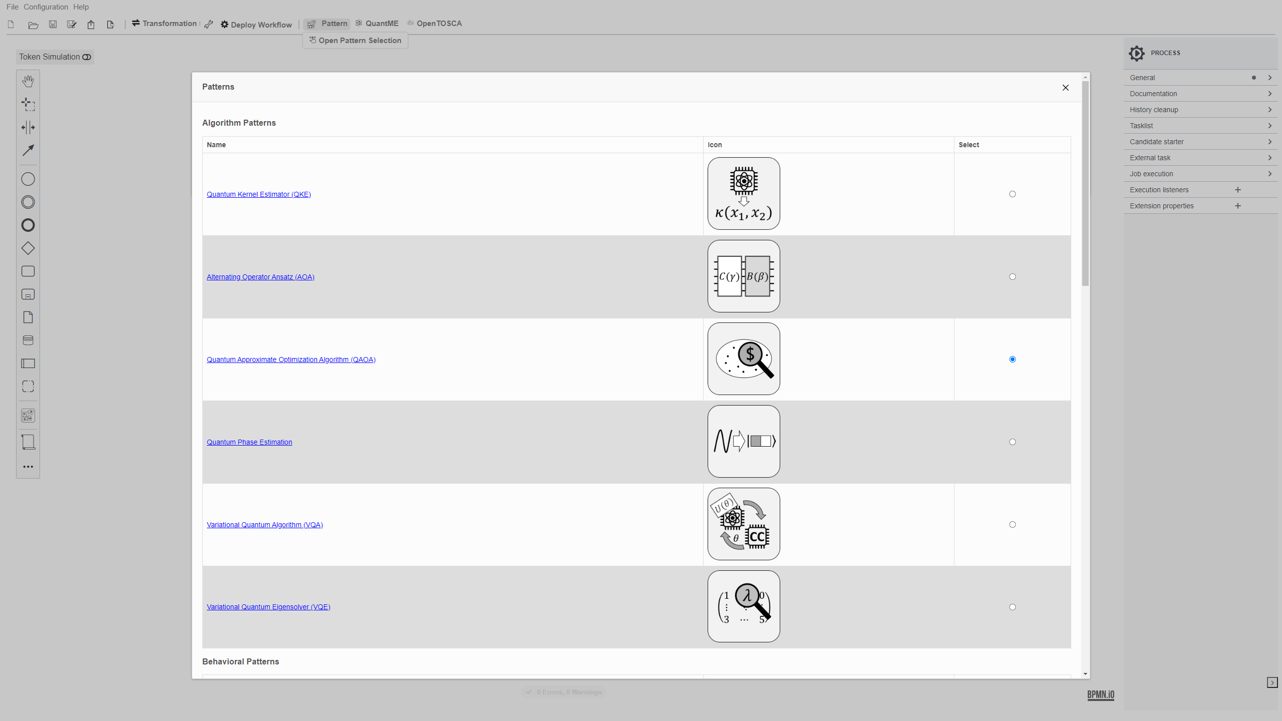

   

3. The screen below displays the current pattern selection, and enables to add another algorithm pattern. For this use case, we only orchestrate a single quantum algorithm, thus, initialize the workflow generation by clicking on Done. Finally, click on Combine Solutions.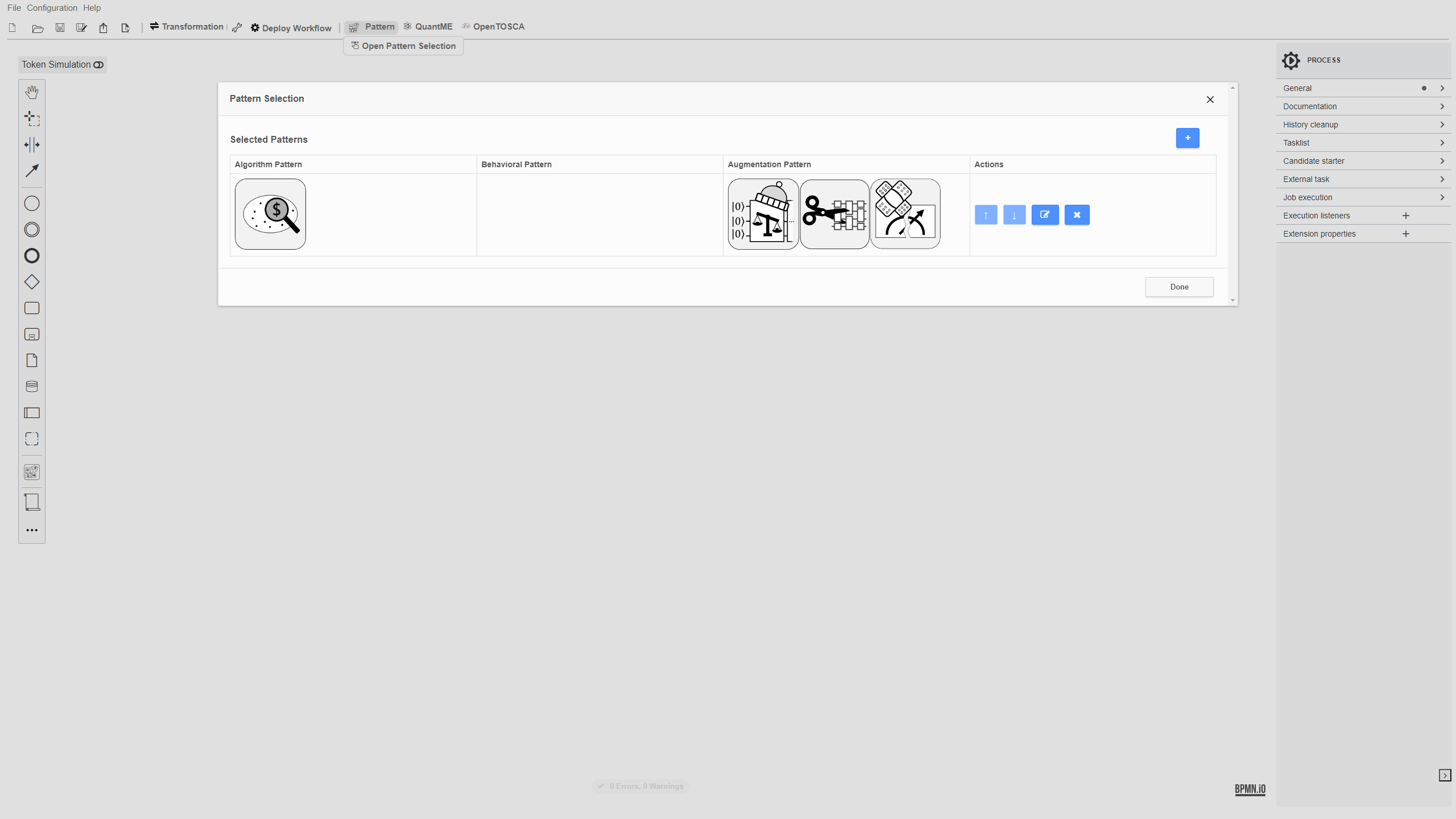

   

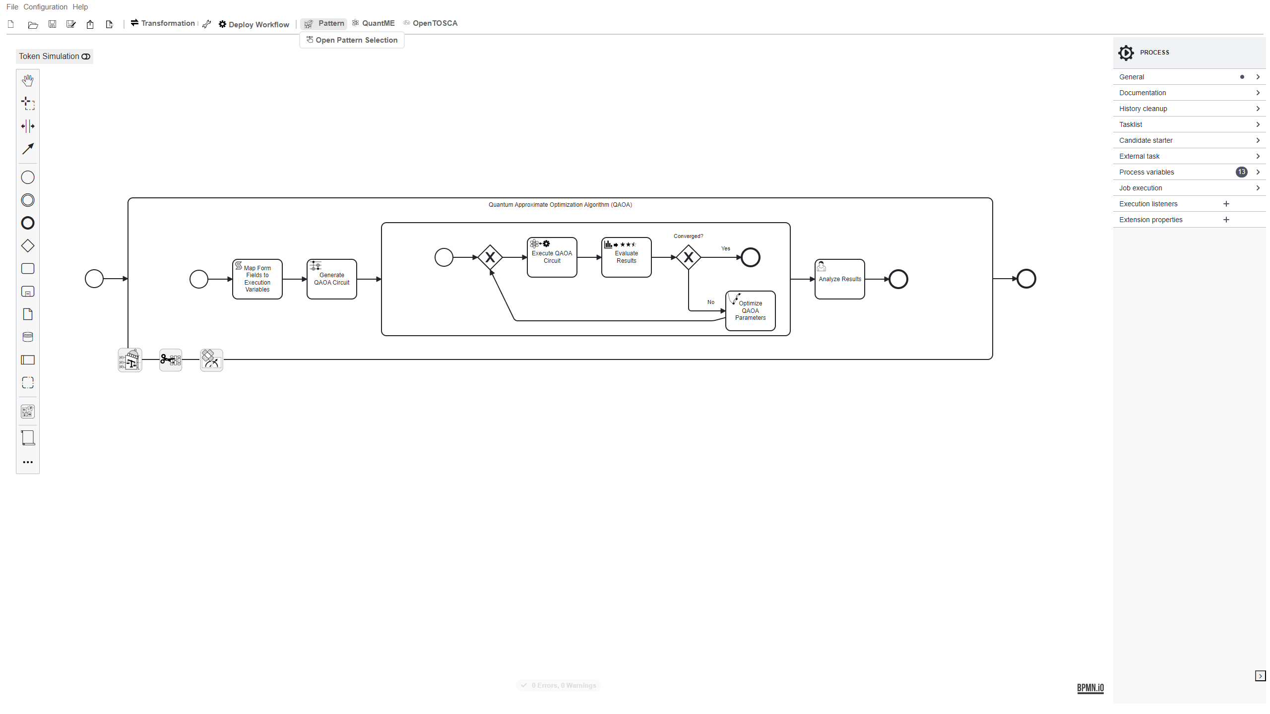
4. The generated quantum workflow is displayed below. It comprises the basic structure of the quantum approximate optimization algorithm, which was loaded from a solution of the corresponding pattern. Additionally, the selected augmentation patterns are attached to the subprocess orchestrating the QAOA algorithm.

   

5. Finally, to transform and execute the generated workflow, follow the steps described in part 1 starting from step 12. Thereby, the transformation also removes the patterns and adds corresponding functionality, leading to a native workflow model for execution.